Transporter Code Generation

Main concept

Transporters are the active components that move data from an Output Buffer (OB) to the next Input Buffer (IB). This step compiles, for every transporter, the program that performs its scheduled data movements with cycle-level accuracy, using the scheduling and addressing information produced by earlier stages.

In most cases each OB instantiates one transporter, although some memory implementations (such as register files) may require two; code is generated independently for every transporter. Because the transporter is a tightly constrained processor — only 15 usable registers and a minimal instruction set — this is essentially a small compiler with three stages: preprocessing, optimisation, and a backend. They all operate on an intermediate representation (IR).

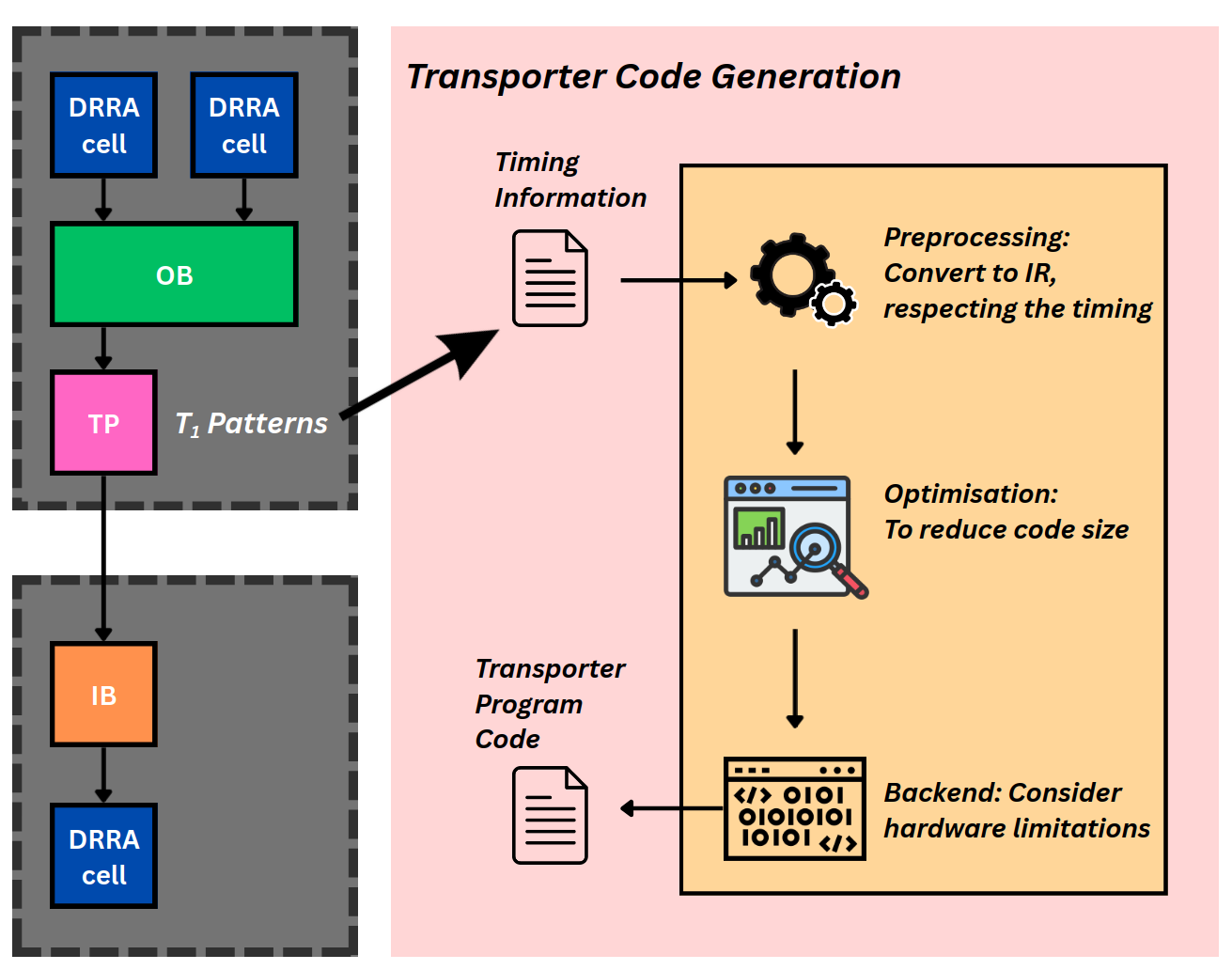Timing information and the T₁ address patterns are converted to IR (preprocessing), optimised to reduce code size, and lowered to transporter program code (backend).

Intermediate Representation (IR)

Since the transporter compiler works under strict timing constraints, the IR makes the clock cycle of every instruction explicit. Each IR entry is a (time, instruction) pair, where the instruction is one of the transporter ISA operations:

time   instruction
0      NOP
1      LDI R3 16
2      MOV R3 R0 0

Preprocessing

Preprocessing converts the scheduling information — a list of (clock cycle, source address, target address) triples — into IR. Each transfer becomes one MOV issued at its scheduled cycle, with the source and target addresses first loaded into registers by LDI instructions. At this stage an unlimited number of registers is assumed (no spilling yet), and the LDI instructions that prepare a MOV are placed at negative time indices, to be scheduled into real cycles later.

input_list      ->  time   instruction
(5, (10, 20))       -4     LDI R4 20
(6, (11, 21))       -3     LDI R3 10
                    -2     LDI R2 21
                    -1     LDI R1 11
                     5     MOV R3 R4 0
                     6     MOV R1 R2 0

Optimisation techniques

These reduce register usage and final code size:

1. Removing redundant registers — if several LDI instructions load the same value, keep one and redirect the others to it.
2. Replacing consecutive MOV with MOVC — if a run of k back-to-back MOVs shares a constant increment c (so source R0 + n·c and destination R1 + n·c for n = 0…k−1), it collapses to a single MOVC R0 R1 R2 k with R2 = c.
3. Reducing register loads with immediate offsets — the MOV immediate field lets the effective addresses be src = R0 + IMM and dst = R1 + IMM, removing some LDI instructions entirely.

Compiler backend

The backend turns the optimised IR into executable transporter code:

1. Removing unused registers — drop LDIs whose register is never used.
2. Tightening the timing in the IR — move the LDI instructions (initially parked before time zero) into available positive time slots, respecting that an LDI must precede the first use of its register and cannot land on an occupied slot or inside a MOVC. Loads are scheduled most-used-register-first (dependency-driven load scheduling).
3. Register allocation — map the unlimited "virtual" registers onto the 15 usable physical registers, using the classic pipeline of liveness analysis → interference-graph construction → graph colouring, spilling when colouring fails. When colouring fails, the spill candidate is chosen by the weighted heuristic score below (see the loop afterwards):

where spillability measures how easy it is to insert reloads, liveRangePressure how long the register stays live, interferenceCost the node's degree in the interference graph, and reuseValue how often the register is used. Each term is multiplied by an adjustable weight.

loop {
    let lives  = liveness(&ir);
    let graph  = interference_graph(&ir, &lives);
    let colours = graph_colouring(&ir, &graph);
    if colours.success { break; }
    transforming_ir(&mut ir, colours.spilled_register);
}

1. Filling NOP instructions — insert NOPs into every empty time slot so the real instructions execute on exactly their scheduled cycles, and append a final NOP 0 so the transporter stalls after it finishes.
2. Final check and code generation — validate value bounds, report the transporter's start time, end time and execution latency back to Sylva (start times may be negative here and are resolved during Control Synthesis), and emit the final binary following the ISA.

Why it matters

Program size directly determines the transporter's instruction-memory area. For regular, affine patterns (e.g. the Sobel example) the MOV→MOVC optimisation can roughly halve the instruction count; for irregular patterns (e.g. most LeNet-5 edges) it rarely applies, and code size is dominated by per-transfer LDI overhead.